부스트캠프 AI Tech 4기
5. Numpy
- -
Numpy (Numerical Python)
numpy는 Numerical Python의 약자로 일반적으로 과학계산에서 많이 사용하는 선형대수의 계산식을 파이썬으로 구현할 수 있도록 도와주는 라이브러리이다.
리스트는 메모리에 주소를 연결하는 구조이기 때문에 굉장히 큰 Matrix에 대한 표현은 효율적이지 않다.
→ 적절한 패키지의 사용이 필요하다.
→ Numpy : Matrix와 Vector와 같은 Array 연산의 사실상의 표준이다.
Numpy의 특징
- 일반 List에 비해 빠르고, 메모리 효율적
- 반복문 없이 데이터 배열에 대한 처리를 지원
- 선형대수와 관련된 다양한 기능 제공
ndarray
▮ array 생성
import numpy as np

array_ex = np.array([1,2,3,4], float)
print(array_ex)
# [1. 2. 3. 4.]

print(type(array_ex))
# <class 'numpy.ndarray'>

print(type(array_ex[1]))
# <class 'numpy.float64'>- np.array 함수를 사용하여 배열을 생성하고 이렇게 생성된 객체를 ndarray라고 부른다.
- numpy는 하나의 데이터 type만 배열에 넣을 수 있다. (List와의 가장 큰 차이점)
▮ Handling shape
- shape : numpy array의 dimension 구성을 반환
- dtype : numpy array의 데이터 type을 반환
array_ex = [[1,2,3],[4,5,6],[7,8,9]]
array_ex = np.array(array_ex)

print(array_ex.shape)
# (3, 3)

print(array_ex.dtype)
# int32
- nbytes : ndarray 객체의 메모리 크기를 반환
np.array([[1,2,3],[4.5, "5", "6"]], dtype=np.float32).nbytes  # 32bits = 4bytes  → 6 * 4bytes
# 24

np.array([[1,2,3],[4.5, "5", "6"]], dtype=np.float64).nbytes
# 48

np.array([[1,2,3],[4.5, "5", "6"]], dtype=np.int8).nbytes
# 6
- reshape : Array의 shape의 크기를 변경, element의 갯수는 동일
matrix_before = [[1,2,3,4],[5,6,7,8]]
np.array(matrix_before).shape
# (2, 4)

np.array(matrix_before).reshape(8,)
# array([1, 2, 3, 4, 5, 6, 7, 8])
row(col)에 -1 size를 적용하면 col(row)에 기반하여 알아서 값을 잡아준다.
np.array(matrix_before).reshape(-1,2).shape
# (4, 2)
- flatten : 다차원 array를 1차원 array로 변환
test_matrix = [[[1,2,3,4],[5,6,7,8]], [[1,2,3,4],[5,6,7,8]]]

test_matrix = np.array(test_matrix)
test_matrix.shape
# (2,2,4)

test_matrix.flatten()
# array([1, 2, 3, 4, 5, 6, 7, 8, 1, 2, 3, 4, 5, 6, 7, 8])
▮ Indexing & Slicing
- list와 달리 행과 열 부분을 나눠서 slicing이 가능함
a = np.array([[1,2,3], [4.5, 5, 6]], int)
a[:,2:]

# array([[3],
#        [6]])
▮ arange
array의 범위를 지정하여 값의 list를 생성
np.arange(0, 5, 0.5)
# array([0. , 0.5, 1. , 1.5, 2. , 2.5, 3. , 3.5, 4. , 4.5])

np.arange(100).reshape(10,10)
# array([[ 0,  1,  2,  3,  4,  5,  6,  7,  8,  9],
#       [10, 11, 12, 13, 14, 15, 16, 17, 18, 19],
#       [20, 21, 22, 23, 24, 25, 26, 27, 28, 29],
#       [30, 31, 32, 33, 34, 35, 36, 37, 38, 39],
#       [40, 41, 42, 43, 44, 45, 46, 47, 48, 49],
#       [50, 51, 52, 53, 54, 55, 56, 57, 58, 59],
#       [60, 61, 62, 63, 64, 65, 66, 67, 68, 69],
#       [70, 71, 72, 73, 74, 75, 76, 77, 78, 79],
#       [80, 81, 82, 83, 84, 85, 86, 87, 88, 89],
#       [90, 91, 92, 93, 94, 95, 96, 97, 98, 99]])
▮ zeros, ones, empty
- zeros : 0으로 가득찬 ndarray 생성
- ones: 1로 가득찬 ndarray 생성
np.zeros(shape=(5,), dtype=np.int8)
# array([0, 0, 0, 0, 0], dtype=int8)

np.ones(shape=(5,), dtype=np.int8)
# array([1, 1, 1, 1, 1], dtype=int8)- empty : shape만 주어지고 비어있는 ndarray 생성 (memory initialization이 되지 않음)
그냥 형태만 잡아주고 아무 값이나 들어가있음
np.empty(shape=(5,), dtype=np.int8)
# array([112,  -1,  -1,  -1,   0], dtype=int8)
▮ something_like
- 기존 ndarray의 shape 크기 만큼 1, 0 또는 empty array를 반환
test_matrix = np.arange(30).reshape(5, 6)
np.ones_like(test_matrix)

# array([[1, 1, 1, 1, 1, 1],
#       [1, 1, 1, 1, 1, 1],
#       [1, 1, 1, 1, 1, 1],
#       [1, 1, 1, 1, 1, 1],
#       [1, 1, 1, 1, 1, 1]])
▮ identity
- 단위 행렬 생성
np.identity(n=3, dtype=np.int8)
# array([[1, 0, 0],
#       [0, 1, 0],
#       [0, 0, 1]], dtype=int8)
▮ eye
- 대각선이 1인 행렬
- 시작값을 k로 정할 수 있음
np.eye(3,5, k=2)
# array([[0., 0., 1., 0., 0.],
# [0., 0., 0., 1., 0.],
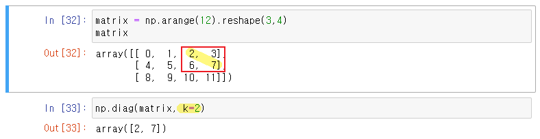
# [0., 0., 0., 0., 1.]])▮ diag
- 대각 행렬의 값만 추출
▮ random sampling
- 데이터 분포에 따른 sampling으로 array를 생성
- np.random.uniform() : 균등분포
np.random.uniform(0, 1, 10).reshape(2,5)
# array([[0.69780063, 0.48244632, 0.94980614, 0.19674234, 0.53045397],
# [0.37472935, 0.35017147, 0.25974474, 0.3344365 , 0.37594652]])- np.random.normal() : 정규분포
np.random.normal(0, 1, 10).reshape(2,5)
# array([[-0.80044157, -1.18365972, -0.26503548,  1.04190843, -0.51664902],
#       [ 0.5493379 ,  1.94129337, -1.74935391,  0.79809954,  1.69312592]])
Operation function
▮ sum
- ndarray의 element들 간의 합 (list의 sum 기능과 동일)
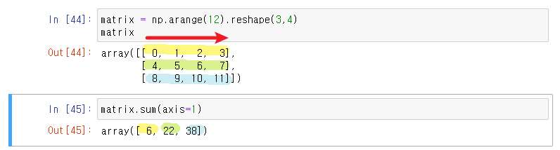
matrix = np.arange(12).reshape(3,4)
matrix
# array([[ 0,  1,  2,  3],
#       [ 4,  5,  6,  7],
#       [ 8,  9, 10, 11]])

matrix.sum(dtype=float)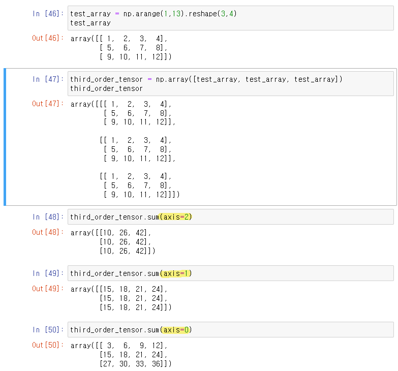
# 66- axis : 모든 operation function을 실행할 때 기준이 되는 dimension 축
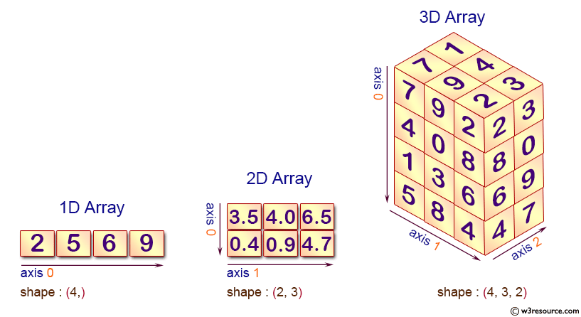
- third order tensor
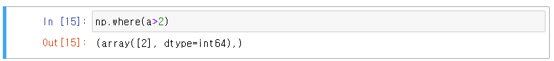
▮ np.where
- np.where(condition, True, False)
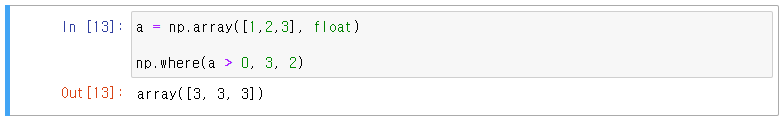
- np.where(condition) → Index값 반환
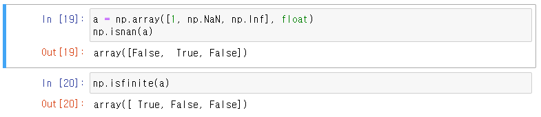
- np.isnan( ) : not a number
- np.isfinite( )
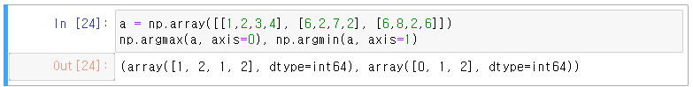
▮ np.argmax , np.argmin
- array내 최대값 / 최소값의 index를 반환
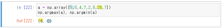
- axis 기반의 반환
boolean & fancy index
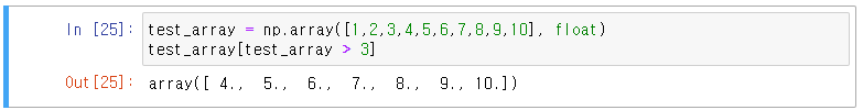
boolean index는 boolean list를 사용하고 fancy index는 integer list를 사용한다.
▮ boolean index
- 특정 조건에 따른 값을 배열 형태로 추출
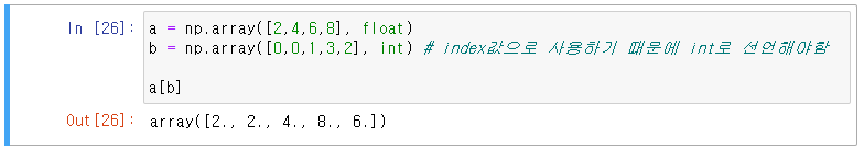
▮ fancy index
- array를 index value로 사용해서 값 추출
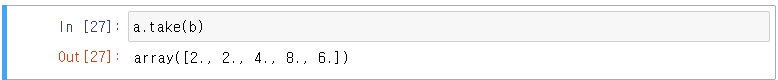
- take( ) : bracket index와 같은 효과
부스트캠프 AI Tech 교육 자료를 참고하였습니다.
728x90
'부스트캠프 AI Tech 4기' 카테고리의 다른 글
| 6. Exception/File/Log handling (1) | 2022.09.23 |
|---|---|
| 5. Python data handling (0) | 2022.09.23 |
| 4. Module and Project/가상환경 (2) | 2022.09.21 |
| 3. 객체지향 프로그래밍 (0) | 2022.09.19 |
| 2. Data Structure/Pythonic Code (0) | 2022.09.18 |
Contents