[Vector Similarity Search] 3 Vector-based Methods for Similarity Search - TF-IDF / BM25 / SBERT

Vector-based  Search. 방식에는 대표적으로 TF-IDF, BM25, 그리고 BERT 기반 방식들이 있다.

• TF-IDF / BM25 → Sparse Vector
• SBERT → Dense Vector

 

1. TF-IDF

TF-IDF 은 명칭처럼 Term Frequency (TF: 단어의 빈도)와 Inverse Document Frequency (IDF: 역 문서 빈도)라는 두 가지를 이용한다.

 

TF : 특정 문서 D에서 특정 단어 q의 등장 횟수

https://www.pinecone.io/learn/semantic-search/

"바나나"라는 단어에 대한 TF를 위와 같이 "바나나" 단어 등장 횟수 / 전체 단어 수로 나타낼 수 있다.

그러나 TF만으로는 흔한 단어와 흔하지 않은 단어에 차별점을 둘 수 가 없다. 위 예시에서 "the'라는 단어의 TF를 구해도 "바나나"와 같기 때문이다.

 

TF-IDF : 특정 단어 q가 등장한 문서의 수의 역수

흔하지 않은 단어에 대해 좀 더 높은 점수를 주기위해 ("the"보다 "banana"에 더 좋은 점수를 주고싶음) IDF를 사용한다. 

https://www.pinecone.io/learn/semantic-search/

 

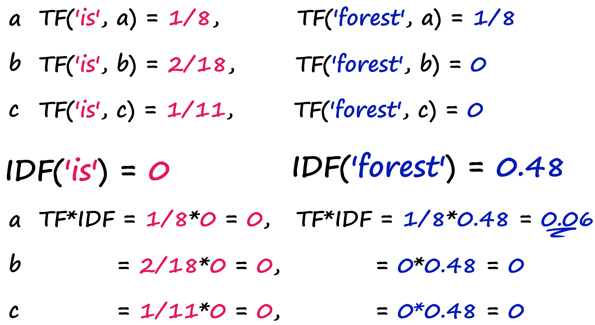
위 그림처럼 a, b, c 라는 세 문서가 있다고 가정하자.

"is" 단어의 IDF 값은 모든 문서에 들어있으므로 0이다.
"forest" 단어의 IDF 값은 a 문서에만 있기 때문에 좀 더 차별점을 줄 수 있을 것이다. 

 

TF-IDF = TF * IDF 

최종적으로 TF-IDF의 값은 TF와 IDF의 값을 곱하여 구할 수 있다.

"is"와 "forest"에 대한 TF-IDF을 구하면 아래와 같다. 

 

 

a = "purple is the best city in the forest".split()
b = "there is an art to getting your way and throwing bananas on to the street is not it".split()
c = "it is not often you find soggy bananas on the street".split()

 

import numpy as np

docs = [a, b, c]

def tfidf(word, sentence):
  freq = sentence.count(word)

  # term frequency
  tf = freq / len(sentence)

  # inverse document frequency
  idf = np.log10(len(docs) / sum([1 for doc in docs if word in doc]))
  
  return round(tf*idf,4)

 

# turn it into vector
vocab = set(a + b + c)

vec_a, vec_b, vec_c = [], [], []

for word in vocab:
  vec_a.append(tfidf(word, a))
  vec_b.append(tfidf(word, b))
  vec_c.append(tfidf(word, c))

 

 

 

2. BM25

TF-IDF도 좋은 방법이지만 a 문서에서 "Ze;da"가 10번 등장하고, b문서에서는 20번 등장하는 경우 a 문서와 Zelda에 대한 관련성이 b 문서의 절반이라고 볼 수는 없을 것이다.

이런 문제점을 해결하기 위해 TF-IDF에 몇 가지 파라미터를 추가한 것이 BM25이다.

https://www.pinecone.io/learn/semantic-search/

 

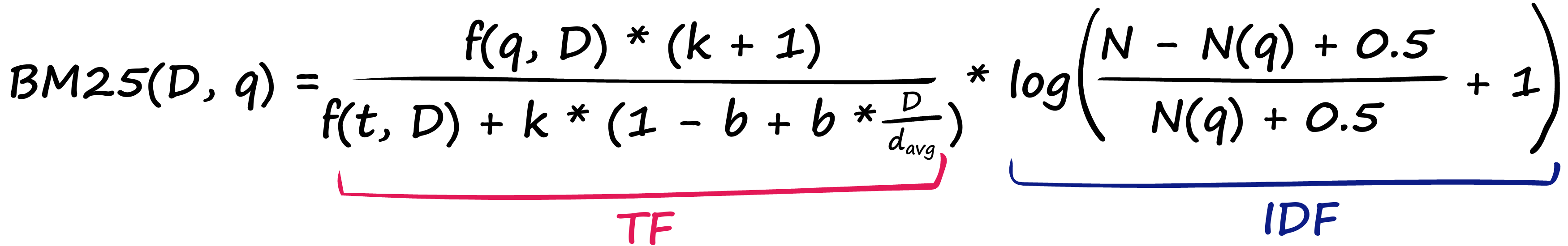
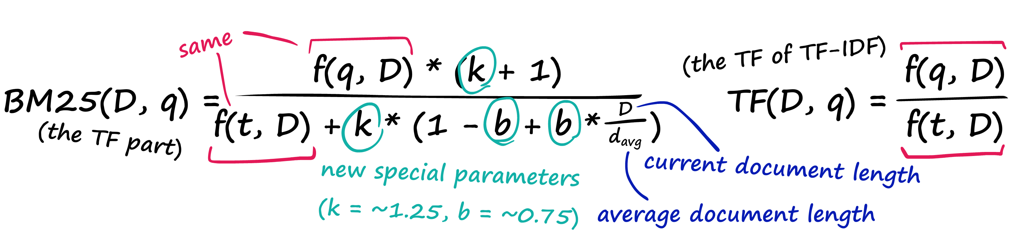
TF 항 부분

https://www.pinecone.io/learn/semantic-search/

 

 

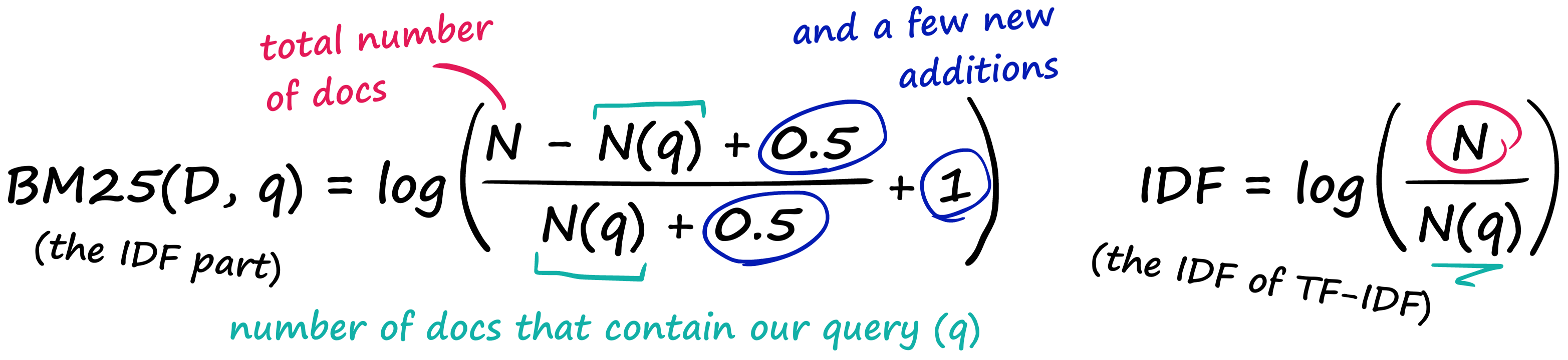
IDF 항 부분

 

TF-IDF는 특정 단어의 수가 증가할 수록 score도 비례해서 증가함을 알 수 있지만, BM25는 그렇지 않음을 알 수 있다.

 

docs = [a, b, c]

def bm25(word, sentence, k=1.2, b=0.75):
  # term frequency
  freq = sentence.count(word)
  avgdl = sum(len(sentence) for sentence in docs) / len(docs)

  tf = (freq * (k+1)) / (len(sentence) + k * (1 - b + b * len(sentence) / avgdl))

  # inverse document frequency
  N = len(docs)
  N_q = sum([1 for doc in docs if word in doc])
  idf = np.log((N - N_q + 0.5) / (N_q + 0.5) + 1)

  return round(tf*idf, 4)

 

 

3. SBERT

Sparse 방식은 Semantic한 정보를 담지 못한다는 것이 단점이다.

BERT는 Dense Vector로 인코딩할 수 있고, 이렇게 표현된 dense vector는 Cosine Similarity 같은 방법을 이용해서 semantic similarity를 측정할 수 있다.

단점은 각 시퀀스가 하나의 벡터가 아니라 512개의 벡터로 표현된다는 점인데, 이 단점을 해결하기 위해 Sentence-BERT가 등장하였다. (BERT는 512,  SBERT는 128)
SBERT는 전체 시퀀스를 단일 벡터로 표현할 수 있다.

Hugging face Library의 sentence_transformer를 사용하면 간단하게 이용할 수 있고,
그렇지 않다면 7개의 문장에 대해서 아래와 같은 차원으로 표현되기 때문에 mean pooling 연산을 통해 변환해준다.

torch.Size([7, 128, 768])

마스킹 연산을 위해 mask array를 만듬

mask = tokens['attention_mask'].unsqueeze(-1).expand(embeddings.size()).float()
mask.shape

torch.Size([7, 128, 768])

 

masked_embeddings = embeddings * mask

 

axis=1을 따라 embedding 값을 합산해 각 768개의 value에 대한 총 값을 계산

summed = torch.sum(masked_embeddings, 1)
summed.shape

torch.Size([7, 768])

 

tensor에서의 각 위치의 attention 값의 개수를 count함

counted = torch.clamp(mask.sum(1), min=1e-9)
counted.shape

torch.Size([7, 768])

 

최종적으로 위에서 구한 값들인 'summed' embedding을 attention으로 주어진 값의 개수로 나누어주는 mean-pooling을 계산한다.

mean_pooled = summed / counted
mean_pooled.shape

torch.Size([7, 768])

 

a = "purple is the best city in the forest"
b = "there is an art to getting your way and throwing bananas on to the street is not it" # similar to 'g'
c = "it is not often you find soggy bananas on the street"
d = "green should have smelled more tranquil but somehow it just tasted rotten"
e = "joyce enjoyed eating pancakes with ketchup"
f = "as the asteroid hurtled toward earth becky was upset her dentist appointment had been canceled"
g = "to get your way you must not bombard the road with yellow fruit" # similar to 'b

 

from sentence_transformers import SentenceTransformer

model = SentenceTransformer("bert-base-nli-mean-tokens")

 

sentence_embeddings = model.encode([a, b, c, d, e, f, g])

 

from sklearn.metrics.pairwise import cosine_similarity
import numpy as np

# calculate similarities
scores = np.zeros((sentence_embeddings.shape[0], sentence_embeddings.shape[0]))

for i in range(sentence_embeddings.shape[0]):
  scores[i, :] = cosine_similarity([sentence_embeddings[i]], sentence_embeddings)[0]

 

 

import matplotlib.pyplot as plt
import seaborn as sns

plt.figure(figsize=(10, 9))
labels = ["a", "b", "c", "d", "e", "f", "g"]
sns.heatmap(scores, xticklabels=labels, yticklabels=labels, annot=True)

 

 

 

---

Reference

https://www.youtube.com/watch?v=ziiF1eFM3_4&list=PLIUOU7oqGTLhlWpTz4NnuT3FekouIVlqc&index=2 

https://wikidocs.net/31698